Disclaimer: This post was written as notes for the Graph Theory series by William Fiset.

Introduction

Types of Graphs

• Undirected Graph (Nodes have no edges)
• Directed graphs (Digraphs or DAGS). There are arrows between nodes u and v

Graphs in this course will be represented as (u, v, w), where w is the weighting. This is for directed graphs.

Trees are undirected graphs with no cycles

Rooted tree is directed, with a root node. Can be an out-tree or an in tree (aborescence vs. anti-aborescence).

DAGS are Directed Acylcic graphs. These are graphs with directed edges and no cycles.

ALL out-trees are DAGS, but NOT ALL DAGs are out-trees.

Bipartite graph is a graph whose vertices can be split into two independent groups U, V such that every edge connects between U and V. Also called “two colorable”, or there is no odd length cycle.

Finally we have complete graph, where there is a unique edge between every pair of nodes. A complete graph with N vertices is known as K_n. Complete graph is worst case, so to test for performance, complete graph is good place to start.

How do we represent graphs on the computer?

• Adjacency matrix: Store all weights in an nxn matrix. Pros are it is efficient in lookup (O(1)) and is very simple. However it requires O(V²) space and iterating time complexity. Fine for dense graphs, but not for sparse graphs.

• Adjacency list: It only stores the nodes to which the current node points. Pros are that it is great for sparse graphs, and iterating over edges is efficient. Main disadvantage is that it is less space efficient on dense graphs, and the the worst case edge weight lookup is O(E).
  i.e.
  A -> [(B,3)]
  B -> [(A,6)]

• Edge List: Simply represent the graph as an unordered list of edges. These can be stored as triplets (u, v, w), which reads as “The cost from node u to node v is w”. This is very simple, but lacks structure. It is great for sparse graphs and iterating over edges is easy. The downside is that it is less space efficient for dense graphs, and the worst case edge weight lookup is O(E).
  i.e.
  [(C, A, 4), (A, C, 1)]

Common Problems and Algorithms

Questions to ask

• Is the graph directed or undirected
• Are the edges of the graph weighted
• Is the graph I will encounter likely to be sparse or dense with edges?
• Should I use adjacency matrix, adjacency list, edge list or some other structure?

Shortest Path

One of the most common problems is the shortest path problem. Many algorithms exist to solve this problem. BFS, Dijkstra’s, Bellman-Ford, Floyd Warshall, A*, and more.

Connectivity

Does there exist a path from node A to Node B? Typical solutions here are union find or simple search algorithm like DFS.

Negative Cycles

Negative cycles are graph cycles that end up with a negative cost. There are places where negative cycles are beneficial. Algorithms to find negative cycles are Bellman-Ford and Floyd-Warshall.

Strongly connected components

Strongly Connected Component can be thought of as self-contained cycles within a directed graph, where every vertex in a given cycle can reach every other vertex in the same cycle. Algorithms to find these components are Tarjan’s and Kosaraju’s.

Traveling Salesman Problem

Give a list of cities and the distances between them, find the shortes possible route that visits each city once and returns back. It is NP-Hard, and has several important applications. Algorithms to solve this are Held-Karp, branch and bound, and many approximation algorithms.

Bridges

A bridge/cut edge is any edge in a graph whose removal increases the number of connected components. A connected component of an undirected graph is a subgraph in which any two vertices are connected to each other by paths, and which is connected to no additional vertices in the supergraph.

Articulation Points

An articulation point/cut vertex is any node in a graph whose removal increases the number of connected components. They are important in graph theory because they often hint at weak points in a graph.

Minimum Spanning Tree

A minimum spanning tree (MST) or minimum weight spanning tree is a subset of the edges of a connected, edge-weighted undirected graph that connects all the vertices together, without any cycles and with the minimum possible total edge weight. Algorithms are Kruskal’s, Prim’s and Boruvka’s.

Network Flow: Max Flow

The question with flow networks is that if we had an infinite input source, how much “flow” can we push through the network? Edge weights represent some sense of capacity, i.e. water through a pipe, or cars through a road. Algorithms are Ford-Fulkerson, Edmonds-Karp & Dinic’s.

Depth First Search (DFS)

DFS is a core algorithm allowing you to traverse a graph. It is easy to code, and has time complexity O(V+E). By itself it isn’t that useful, but can be very useful for other tasks.

Note that in DFS, you can’t revisit the same node. So if you either visit a leafnode or get to a visited node, you have to backtrack. You can have multiple ways to do DFS.

1
2
3
4
5
6
7
8
9
10
11
12
13
14
15
16
# Global or class scope variables
n = number of nodes in graph
g = adjacency list representing graph
visited = [false, ..., false] # size n

function dfs(at):
    if visited[at]: return
    visited[at] = true

    neighbours = g[at]
    for next in neighbours:
        dfs(next)

# Start DFS at node zero
start_node = 0
dfs(start_node)

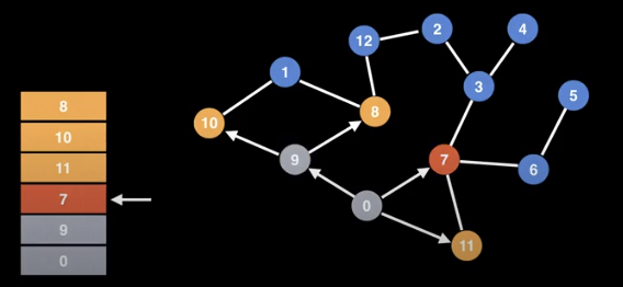
Finding Connected Components

Can we label each node in a component with the same id value? We can use DFS to identify components.

1. First makes sure all the nodes are labeled from [0, n) where n is the number of nodes.
2. Start at every node, unless that node has already been visited, marking all nodes in the same search with the same value.

1
2
3
4
5
6
7
8
9
10
11
12
13
14
15
16
17
18
19
20
21
# Global or class scope variables
n = number of nodes in the graph
g = adjacency list representing graph
count = 0
components = empty integer array # size n
visited = [false, ..., false] # size n

function findComponents():
    for (i=0; i<n; i++):
        if !visited[i]:
            count++
            dfs(i)
        return (count, components)

function dfs(at):
    if visited[at] return
    visited[at] = true

    for (node : g[at]):
        if !visited[node]:
            dfs(node)

What else can DFS do?

• Comput a graphs MST
• Detect and find cycles in a graph
• Check if a graph is bipartite
• Find strongly connected components
• Topologically sort the nodes of a graph
• Find bridges and articulations points
• Find augmenting paths in a flow network
• Generate mazes

Breadth First Search (BFS)

Another fundamental search algorithm, runs with a time complexity of O(V + E). It is particularly useful for finding the shortest path on unweighted graphs.

Unlike DFS, we will visit all of the neighbours first instead of drilling down to the leaf nodes. It explores in a layered fashion by maintaining a queue.

BFS uses a queue to track where to go next. Upon reaching a new node, it adds it to the queue so we can visit it later. We will need some sort of data structure that shows which nodes we have visited so we don’t revisit.

1
2
3
4
5
6
7
8
9
10
11
12
13
14
15
16
17
18
19
20
21
22
23
24
25
26
27
28
29
30
31
32
33
34
35
36
37
38
39
40
41
42
43
44
45
# Function that calculates shortest path
# Global/class scope variables
n = number of nodes in the graph
g = adjacency list representing unweighted graph

# s = start node, e = end node, and 0 <= e, s < n
def bfs(s, e):

    # Do a BFS starting at node s
    prev = solve(s)

    # return reconstructPath(s, e, prev)

def solve(s):
    q = queue data structure
    q.enqueue(s)

    visited = [false, ..., false] # size n
    visited[s] = true

    prev = [null, ..., null] # size n
    while !q.isEmpty():
        node = q.dequeue()
        neighbours = g.get(node)

        for (next : neighbours):
            if !visited[next]:
                q.enqueue(next)
                visited[next] = true
                prev[next] = node
    return prev

def reconstructPath(s, e, prev):

    # Reconstruct the path going backward from e
    path = []
    for (at = e; at != null; at = prev[at]):
        path.add(at)

    path.reverse # path[::-1]

    # If s and e are connected return the path
    if path[0] == s:
        return path
    return []

Breadth First Search (BFS) Grid Shortest Path

Motivation: A suprising number of problems can be represented using a grid. Grids are implicit graph, because we can determine neighbours based on the grid.

Common approach is to convert to adjacency list/matrix. Cells are connected left right, up and down.

1. Label all cells in the grin with numbers [0, n)
2. Construct an adjacency list and matrix based on the grid
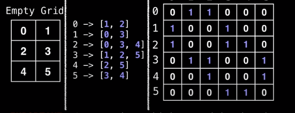
3. Then we can run whatever graph algorithm we want to run.

However we can usually avoid transformations due to the structure of the graph itself.

1
2
3
4
5
6
7
8
9
10
11
12
13
# Define the direction vectors for north, south, east, and west
dr = [-1, +1, 0, 0]
dc = [0, 0, +1, -1]

for (i = 0; i < 4; i++):
    rr = r + dr[i]
    cc = c + dc[i ]

    # Skip invalid cells. Assume R 
    # and C for the number of rows and columns
    if rr < 0 or cc < 0: continue
    if rr >= R or cc >= C: continue
    # (rr, cc) is neighbour of cell (r, c)

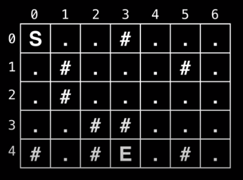
Real Example

You are trapped in a dungeon and need to find the quickest way out. The dungeon is composed of unit cubes which may or may not be filled with rock. It takes one minute to move one unit north, south, east, and west. You cannot move diagonally and the maze is surrounded by solid rock on all sides.

Is an escape possible? If yes, how long will it take?

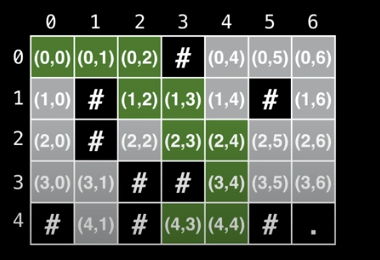
Alternative State Representation

Right now we are storing the values as either an (x, y) pair or an object representation.

An alternative approach is to use one queue for each dimension. When we do this however, we need to make sure that we enqueue and dequeue elements all at the same time.

1
2
3
4
5
6
7
8
9
10
11
12
13
14
15
16
17
18
19
20
21
22
23
24
25
26
27
28
29
30
31
32
33
34
35
36
37
38
39
40
41
42
43
44
45
46
47
48
49
50
51
52
53
54
55
56
57
58
59
60
# Global/class scope variables
R, C = ... # R = # rows, C = # columns
m = ... # The input character grid of size R x C
sr, sc = ... # Starting point coordinates
rq, cq = ... # Empty Row Queue and Column Queue

# Variables used to track the number of steps taken
move_count = 0
nodes_left_in_layer = 1
nodes_in_next_layer = 0

# Variable used to track whether the 'E' character
# ever gets reached during BFS
reached_end = false

# R x C matrix of false values used to track whether
# the node at position (i, j) has been visited
visited = ...

dr = [-1, +1, 0, 0]
dc = [0, 0, +1, -1]

def solve():
    rq.enqueue(sr)
    cq.enqueue(sc)
    visited[sr][sc] = true
    while rq.size() > 0:
        r = rq.dequeue()
        c = cq.dequeue()
        if m[r][c] == 'E':
            reached_end = true
            break
        explore_neighbours(r, c)
        node_left_in_layer--
        if nodes_left_in_layer == 0:
            nodes_left_in_layer = nodes_in_next_layer
            nodes_in_next_layer = 0
            move_count++
    if reached_end:
        return move_count
    return - 1

def explore_neighbours(r, c):
    for (i = 0; i < 4; i++):
        rr = r + dr[i]
        cc = c + dc[i ]

        # Skip invalid cells. Assume R 
        # and C for the number of rows and columns
        if rr < 0 or cc < 0: continue
        if rr >= R or cc >= C: continue
        # (rr, cc) is neighbour of cell (r, c)

        if visited[rr][cc]: continue
        if m[rr][cc] == #: continue

        rq.enqueue(rr)
        cq.enqueue(cc)
        visited[rr][cc] = true
        nodes_in_next_layer++

Introduction to Tree Algorithms

What is a tree? A tree is an undirected graph with no cycles.

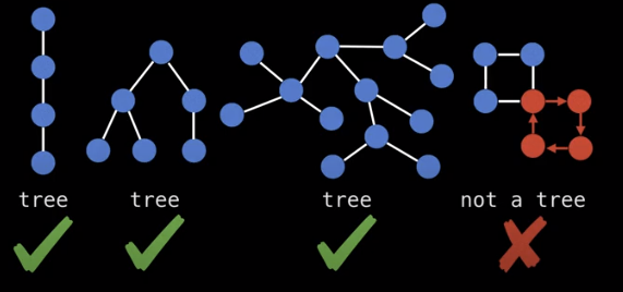
There is an even easier way to check if a graph is a tree. Each tree has exactly n nodes, and n-1 edges

Trees in the wild

• File system
• Social heirarchies
• Prefix Notation
• Webpages (DOM)
• Game Theory to model decisions and courses of action, i.e. prisoner’s dilemma
• Probability trees
• Taxonomy
• etc…

Storing undirected trees

You can store trees by doing the following

1. Label from [0, n)
2. Setup storage representation
   1. Edge list
      1. This is super fast
      2. Easy to iterate over
      3. Lacks structure to query neighbours
   2. Adjacency List
      1. Mapping from node to labels
      2. Easy to find neighbours
   3. Adjacency Matrix
      1. Easy
      2. Huge, huge waste of space (n²)

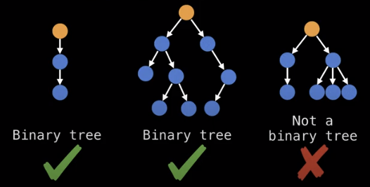
Rooted Trees are directed trees, you can have an out-tree (arborescence) or an in-tree (anti-arborescence).

Related to root trees are binary trees which can have at most two child nodes.

Binary search trees are binary trees which satisfy the binary search tree invariant which is:

x.left.value <= x.value <= x.right.value

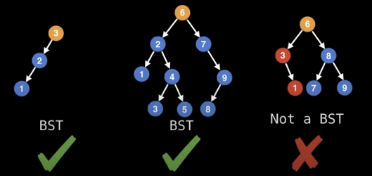
Note how the last tree above is not a binary search tree because it breaks the invariant.

We can also make the invariant strict, to avoid duplicate values.

Storing rooted trees

In practice you always maintain a pointer to the root node so you can access the tree and all of its content.

Each node also has a list of all its children, known as child nodes. Leaf nodes do not have any children.

Sometimes it is also useful to have a pointer to a node’s parent node so that you can traverse up the tree. This is not usually necessary, because you can access the node on the recursive callback.

If tree is an n-ary tree, we can also store it as a flattened array.

Here, each node has an assigned index position based on where it is in the tree. Here, even if there are missing nodes, they have an index in the array.

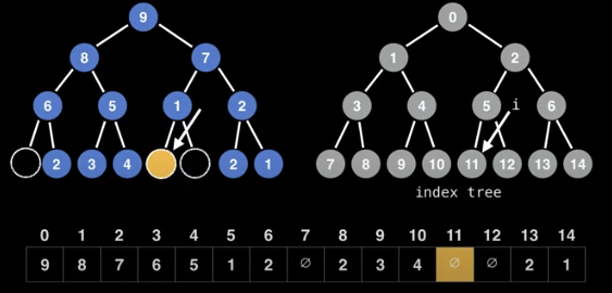
In this representation, we can calculate the indices of nodes as follows

• left node: 2*i + 1
• right node: 2*i + 2

Reciprocally, the parent of node i is:

• floor((i-1)/2)

Beginner Tree Algorithms

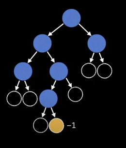
Problem 1

Find the sum of all the leaf node values in a tree.

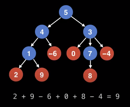
We can do a searching algorithm algorithm like BFS or DFS.

1
2
3
4
5
6
7
8
9
10
11
12
13
14
15
16
17
# Sums up leaf node values in a tree.
# Call function like: leafSum(root)
def leafSum(node):
    # Handle empty tree case
    if node == null:
        return 0
    
    if isLeaf(node):
        return node.getValue()
    
    total = 0
    for child in node.getChildNodes():
        total += leafSum(child)
    return total

def isLeaf(node):
    return node.getChildNodes().size() == 0

Problem 2

Find the height of a binary tree. The height of a tree is the number of edges from the root to the lowest leaf.

Leaf nodes have a height of 0

We can set up a height function h(x)

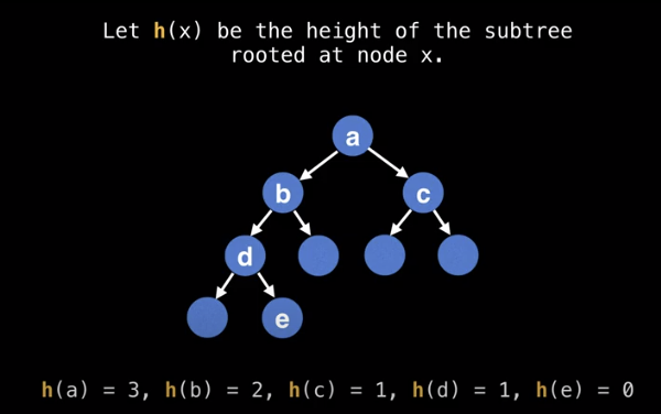
We can set up a recurrence relation as follows.

h(x) = max(h(x.left), h(x.right)) + 1

Note that we are recursively computing the height of the subtrees. Here is the recursive pseudocode

1
2
3
4
5
6
7
8
9
10
11
12
# The height of a tree is the number of
# edges from the root to the lowest leaf.
def treeHeight(node):
    # Handle empty tree case
    if node == null:
        return -1

    # Identify leaf nodes and return zero
    if node.left == null and node.right == null:
        return 0

    return max(treeHeight(node.left), treeHeight(node.right)) + 1

Note, that we could do the following, and the algorithm will still work correctly

1
2
3
4
5
6
7
8
# The height of a tree is the number of
# edges from the root to the lowest leaf.
function treeHeight(node):
    # Handle empty tree case
    if node == null:
        return -1

    return max(treeHeight(node.left), treeHeight(node.right)) + 1

This works because we are effectively adding extra “null nodes” to the tree and correcting for the heigh by returning -1.

Keep in mind, that we can also dynamically keep track of the height of a tree when we are constructing it, although that may not always be possible.

Rooting a Tree

The motivation for rooting a tree is that often if can help to add structure and simplify the problem you are trying to solve.

Conceptually, rooting a tree is like picking up the tree by a specific node, and having all the edges point downwards.

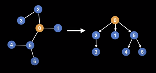
Note that you can root a tree using any nodes, but not every selection will be well balanced. In some situations, it is useful to keep a reference to the parent node, in order to walk up the tree.

One way to root a tree, is to use depth first search.

1
2
3
4
5
6
7
8
9
10
11
12
13
14
15
16
17
18
19
20
21
22
23
24
25
26
27
28
29
30
# TreeNode object structure
class TreeNode:
    # Unique integer id to identify this node
    int id;

    # Pointer to parent TreeNode reference. Only the 
    # root node has a null parent TreeNode reference.
    TreeNode parent;

    # List of pointers to child TreeNodes.
    TreeNode[] children;

# g is the graph/tree represented as an adjacency
# list with undirected edges. If there's an edge between
# (u, v) there's also an edge between (v, u).
# rootId is the id of the node to root the tree from.
def rootTree(g, rootId = 0):
    root = TreeNode(rootId, null, [])
    return buildTree(g, root, null)

# Build tree recursively using depth first
def buildTree(g, node, parent):
    for childId in g[node.id]:
        # Avoid adding an edge pointing back to the parent
        if parent != null and childId == parent.id:
            continue
        child = TreeNode(childId, node, [])
        node.children.add(child)
        buildTree(g, child, node)
    return node

Tree center(s)

Finding a center of a tree is a useful way to select a node to root the tree. Note here that there may be more than one tree center, but there can’t be more than two.

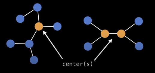
The center of a tree is always the middle vertex or middle two vertices in every longest path along the tree.

Another approach is to peel away the outer layers of the tree, until we reach the center.

Steps

1. Compute the degree of each node (the number of nodes a specific node is connected to)
2. Prune edges, and update degree values
3. Keep doing 1. and 2. until we reach the center/centers

1
2
3
4
5
6
7
8
9
10
11
12
13
14
15
16
17
18
19
20
21
22
# g = tree represented as an undirected graph
def treeCenters(g):
    n = g.numberOfNodes()
    degree = [0, 0, ..., 0] # size n
    leaves = []
    for (i = 0; i < n; i++):
        degree[i] = g[i].size()
        if degree[i] == 0 or degree[i] == 1:
            leaves.add(i)
            degree[i] = 0
    count = leaves.size()
    while count < n:
        new_leaves = []
        for (node : leaves):
            for (neighbour : g[node]):
                degree[neighbour] = degree[neighbour] - 1
                if degree[neighbour] == 1:
                    new_leabes.add(neighbour)
            degree[node] = 0
        count += new_leaves.size()
        leaves = new_leaves
    return leaves # center(s)